Change or Continuity?

Topic Modeling of Thailand in Transition

Introduction

Do newspaper articles that are published before and after the occurrence of a regime transition differ systematically in terms of their topic coverage and content? Conventional wisdom holds that media patterns are likely to be responsive to changes in government and political institutions as a state undergoes a regime transition. However, it is difficult to make well-informed inferences about how such process occurs in practice and to understand its implications without a comprehensive content analysis of a large sample of newspaper articles that are published during periods of transitions.

Utilizing an original dataset containing all political news published from 2013 to 2015 by The Nation, an English-language daily newspaper in Thailand, this post explores the relationship between regime transition and the media. Specifically, I analyze newspaper articles that were published under democratic rule (pre-May 2014 coup) and those that were published under military rule (post-May 2014 coup), using latent Dirichlet allocation (LDA) to discover latent topics that are associated with the corpus and to trace the prevalence of these topics amidst a regime transition. Then, leveraging the topic labels generated by the model, I conduct a series of quantitative content analyses for assessing the frequencies of words and measuring the sentiments associated with a given topic over time and across the cutoff point of the May 2014 coup d’état.

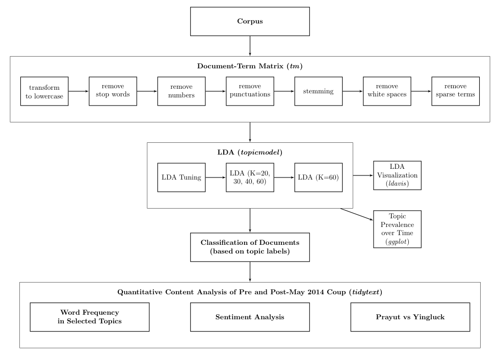
A Flow Chart of Methodology

Data Collection and Pre-Processing

All newspaper articles published by The Nation from 2013 to 2015 were collected from the Nexis Uni database via Rselenium, which extracted relevant information such as the headline, content, and date. The search query used in this process of data collection is “thailand”. The rationale behind this data collection strategy is to gather as many articles by The Nation as possible since in theory there is no a priori justification to regard one type of articles as more or less relevant to the analysis of the effects of regime type than another. However, in practice, due to time constraints and computational efficiency, only articles that contain a set of keywords that are predictive of their political content were retained for the analysis.

These keywords include: “politic*”, “gov*”, “democ*”, “Yingluck”, “junta”, “Prayut”, “Pheu”, and “NCPO”. Any articles that contain at least one of these words or word stems are selected. One problem with this strategy is that the keyword selection process is potentially arbitrary, inadequate for minimizing false positives and lacking in terms of intercoder reliability. An alternative strategy would be to use a computer-assisted approach offered by King, Lam and Roberts (2017), relying on an unsupervised selection of documents in search set, S, into target set, T, based on a hand-coded reference set R. However, in this project, the dictionary-based approach is selected for computational efficiency. This process yields a total of 20,703 articles (D) where the average length is 580 words.

Data Collection

# Set working directory
setwd("~/polisci490/Project")

# Load packages
packages <- c("xml2","rvest", "dplyr", "tm", "tidytext", "ggplot2", "SnowballC", "tidyverse", "lubridate", "stringr", "httr", "SnowballC", "wdman", "RSelenium", "tcltk", "XML", "topicmodels", "stringi", "LDAvis", "slam", "ldatuning", "kableExtra", "widyr", "igraph", "ggraph", "fmsb", "pander")

load.packages <- function(x) {
  if (!require(x, character.only = TRUE)) {
    install.packages(x, dependencies = TRUE)
    library(x, character.only = TRUE)
  }
}

lapply(packages, load.packages)

########## Data Collection (Don't Run this!!)########## 

# Run Selenium Server
rD <- rsDriver()
remDr <- remoteDriver(remoteServerAddr = "localhost" 
                      , port = 4567L
                      , browserName = "chrome"
)


# Log in
remDr$open()
remDr$navigate("https://advance-lexis-com.turing.library.northwestern.edu/api/permalink/920dc8d1-6625-47c3-bdd4-b1c073f28f78/?context=1516831")
username <- remDr$findElement(using = 'id', value = "IDToken1")
password <- remDr$findElement(using = 'id', value = "IDToken2")
username$sendKeysToElement(list("id"))
password$sendKeysToElement(list("pass", "\uE007"))

# click

continue <- remDr$findElement(using = "xpath", "//*[@id='33Lk']/div/div/div/section/div/menu/input[1]")
continue$clickElement()

# Initializing an empy dataframe
# df <- data.frame(title=NULL, text=NULL, date=NULL, length=NULL)

# Scraping

remDr$setTimeout(type = "page load", milliseconds = 100000)
remDr$setImplicitWaitTimeout(milliseconds = 100000)
for(i in 1:20000){
  tryCatch({
    title <- remDr$findElement(using = "id", "SS_DocumentTitle")
    date <- remDr$findElement(using = "xpath", "//*[@id='document']/section/header/p[3]")
    length <- remDr$findElement(using = "xpath", "//*[@id='document']/section/span/div[2]")
    body <- remDr$findElement(using = "xpath", "//*[@id='document']/section/span")
    
    preptext <- function(x){ data.frame(matrix(unlist(x), nrow=length(x), byrow=T))}
    
    title_txt <- preptext(title$getElementText())
    date_txt <- preptext(date$getElementText())
    length_txt <- preptext(length$getElementText())
    body_txt <- preptext(body$getElementText())
    
    docdf <- data.frame(title=title_txt, text=body_txt, date=date_txt, length=length_txt)
    df <- rbind(df, docdf)
    
    Sys.sleep(sample(1:4, 1))
    next_page <- remDr$findElement(using="xpath", "//*[@id='_gLdk']/div/form/div[1]/div/div[14]/nav/span/button[2]")
    next_page$highlightElement()
    next_page$clickElement()
    
  }, error=function(e){
    Sys.sleep(sample(1:10, 1))
    title <- remDr$findElement(using = "id", "SS_DocumentTitle")
    date <- remDr$findElement(using = "xpath", "//*[@id='document']/section/header/p[3]")
    length <- remDr$findElement(using = "xpath", "//*[@id='document']/section/span/div[2]")
    body <- remDr$findElement(using = "xpath", "//*[@id='document']/section/span")
    
    preptext <- function(x){ data.frame(matrix(unlist(x), nrow=length(x), byrow=T))}
    
    title_txt <- preptext(title$getElementText())
    date_txt <- preptext(date$getElementText())
    length_txt <- preptext(length$getElementText())
    body_txt <- preptext(body$getElementText())
    
    docdf <- data.frame(title=title_txt, text=body_txt, date=date_txt, length=length_txt)
    df <- rbind(df, docdf)
    
    Sys.sleep(sample(1:4, 1))
    next_page <- remDr$findElement(using="xpath", "//*[@id='_gLdk']/div/form/div[1]/div/div[14]/nav/span/button[2]")
    next_page$highlightElement()
    next_page$clickElement()
  })}

Data Pre-processing

# Assign variable names
names(df) <- c("title", "text", "date", "wordcount")

# Set date
df$date <- mdy(as.character(df$date))

# Clean content
df$text <- gsub("^.*Body\n|Classification.*$","", as.character(df$text))
df$text <- gsub( " *@.*?; *", "", as.character(df$text))
df$text <- gsub( "*â€", "", as.character(df$text))
df$text <- gsub( "*–", "", as.character(df$text))
df$title <- gsub( " *@.*?; *", "", as.character(df$title))
df$title <- gsub( "*â€", "", as.character(df$title))
df$title <- gsub( "*–", "", as.character(df$title))
df$title <- gsub( "*#124", "", as.character(df$title))
df$text <- gsub( "*#124", "", as.character(df$text))
df$text <- gsub("*Prayuth", "Prayut", as.character(df$text)) # Prayut & Prayuth
df$title <- gsub("*Prayuth", "Prayut", as.character(df$title)) # Prayut & Prayuth

# Get word count
df$wordcount <- as.numeric(gsub("Length: | words", "", df$wordcount))

# Filter for politics
keyword <- c("politic*", "gov*", "democ*", "Yingluck", "junta", "Prayut", "Pheu", "NCPO")
pattern <- grepl(paste(keyword, collapse = "|"), df$text)
df <- df[pattern, ]

# select date Jan 2013 - Sep 2015
df.2013 <- filter(df, date >= "2013-01-01" & date < "2016-01-01")

# Remove duplicate rows
df.2013 <- distinct(df.2013)

# Add doc_id
df.2013 <- df.2013 %>% mutate(doc_id = seq.int(nrow(df.2013)))

# Finalize dataset
df.2013 <- df.2013 %>% select(doc_id, text, everything())

Table 1: Data Structure

Using the tm package, I converted the data to a corpus object, transformed words to lower cases and removed stop words, numbers, punctuations, followed by stemming and removing white spaces. Then, I parsed the corpus to a document-term matrix with articles as documents in the rows and terms in the columns. Finally, sparse terms that appear in less than 0.01 of all documents are removed.

This process yields 2,946 unique word stems (W) for the analysis, producing a 20,703 by 2,946 input matrix which contains 3,384,956 non-sparse entities for the topic model. One consideration that must be taken into account is that the topic models may be sensitive to these pre-processing choices (Denny and Sperling 2017). In theory, transforming to lower cases, removing numbers and removing punctuations should not significantly alter the findings of this project, whereas stemming and removing stop words may result in a loss of information or generate noise in the model. Although a comparison of findings with different preprocessing choices is not presented here, this can be implemented in future work to test the robustness of the topic models.

# Create corpus
nation <- VCorpus(DataframeSource(df.2013))

# Pre-process + generate document-term matrix
nation.dtm <- nation %>% 
  tm_map(content_transformer(tolower)) %>%
  tm_map(removeWords, stopwords("english")) %>%
  tm_map(removeNumbers) %>%
  tm_map(removePunctuation) %>%
  tm_map(stemDocument) %>%
  tm_map(stripWhitespace) %>%
  DocumentTermMatrix() %>%
  removeSparseTerms(sparse = 0.99)

Latent Dirichlet Allocation (LDA)

Following Blei, Ng and Jordan (2003), I employ latent Dirichlet allocation (LDA) as an unsupervised method for learning the topics associated with the newspaper articles. One advantage that LDA offers over unigram models is that it treats documents as “random mixtures over latent topics, where each topic is characterized by a distribution over words” (996). An important implication of this probabilistic feature is that each document is allowed to represent multiple topics instead of being restricted as discrete entities to a single topic. It must be noted, however, that utilizing LDA for dimensionality reduction entails making a number of modeling assumptions, two of which will be discussed here.

Exchangeable and Static

First, LDA assumes “bag-of-words” such that words in a document are treated as exchangeable. Hence, not only are the words themselves treated as infinitely exchangeable across documents and topics, word ordering is also ignored, despite the fact that such ordering may be highly informative and meaningful for the generative process through which words are assigned probability of being associated to different topics.

Second, it assumes that topics are static across time, while the occurrence of topics may vary with time. That is, the number of topics is assumed to be fixed and the parameters which characterize these topics are treated as time-invariant, when in fact topics may emerge and disappear or constitute themselves differently over time. It is important to recognize these limitations because they inform the extent to which the LDA can be relied upon for representing the documents in the corpus. I also considered using structural topic modeling (STM) as an alternative strategy. However, given the lack of available covariates on which to condition the topic model on, LDA is chosen for the study. One disadvantage of this is that the model is likely to be noisy given that informative metadata such as news category is not included as part of the modeling. Given that this problem could be exacerbated in a model that poorly fits the data, it is crucial to determine the optimal number of topics for fitting the LDA.

Choosing the Number of Topics (k)

For LDA, the dimensionality of the Dirichlet distribution, k, is assumed to be known and fixed. Hence, selecting an optimal value of k is critical for obtaining a topic model that best describes the data. Among the possible strategies for determining the optimal parameters for fitting LDA models, I use LDAtuning, an R package that estimates the performance of LDA models using Gibbs sampling and reports the performance based on four different metrics: harmonic means (Griffith and Steyvers 2004), cosine distance (Cao et. al. 2009), Kullback-Leibler divergence (Arun et. al. 2010) and Jensen-Shannon divergence (Deveaud et. al. 2014). Note, however, that this method does not involve validation, cross-validation, or splitting the data into train and test set, which is typically the case for perplexity-based methods. I fit 9 models from 20 to 100 topics, increasing k by 10.

Figure 1 shows the effects on the four metrics when varying parameter k by 10. According to these metrics, the performance of LDA models improves most significantly when moving to 40 and 60 topics. In addition to these objective measures, I also evaluate the models based on their interpretability. Among models with k=20, 30, 40 and 60, the model with 60 topics is least perplexing to the human coder and most informative in terms of generating topic labels that are helpful for making an informed guess as to what each topic is about. Only the findings based on this model is reported in this post.

result <- FindTopicsNumber(
  nation.dtm,
  topics = seq(from = 20, to = 200, by = 10),
  metrics = c("Griffiths2004", "CaoJuan2009", "Arun2010", "Deveaud2014"),
  method = "Gibbs",
  control = list(seed = 77),
  mc.cores = 2L,
  verbose = TRUE
)
FindTopicsNumber_plot(result)

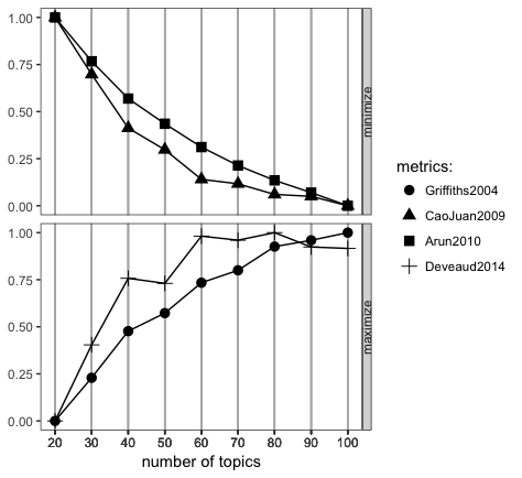
Figure 1: LDA Tuning

Topic Model (2013-2015)

LDA is performed on the entire corpus comprising of political news from 2013 to 2015 with parameter k = 60. This generates a 60 by 2,946 matrix containing the log odds of word being associated with a given topic, and a 20,703 by 60 matrix containing the probabilities of a document being associated with a given topic.

The objective of the topic modeling is to discover latent topics in the corpus that characterize a broad range of issues that have major political implications such as “Human Rights,” “Corruption,” and “Political Conflict,” in other words, topics that are likely to be affected by or correlated with the transition observed in May 2014. Hence, the topics must be sufficiently fine-grained, capturing beyond linguistic or broad categorical differences, but also general enough to maintain salience over time. Most importantly, the topics should contain high semantic validity such that the relationship between words that are generated by each topic are meaningful.

Table 2 provides a list of topics and keywords associated with each topic. The substantive labels for each topic are provided after reviewing the keywords which best distinguish one topic from another. These keywords are selected and sorted based on their rank as determined by the value of the log odds of word being associated with a given topic. The output of the model is also parsed through R package ldavis, creating an interactive web-based visualization which is accessible below.

### LDA
mod.out.60 <- LDA(nation.dtm, k=60, control = list(seed=6))
class(mod.out.60) <- "LDA"
tidy(mod.out.60)

### Generate topic labels (top 30 terms)
nation.topics <- topics(mod.out.60, 1)
nation.terms <- as.data.frame(terms(mod.out.60, 30), stringsAsFactors = FALSE)

### Table
topic_list <- data.frame(t(nation.terms))
topic_list <- within(topic_list, x <- paste(X1, X2, X3, X4, X5, X6, X7, X8, X9, X10, X11, X12, X13, X14, X15, X16, X17, X18, X19, X20, sep=", ")) %>% select(x)
colnames(topic_list) <- NULL
topic_list <- tibble::rownames_to_column(topic_list)
colnames(topic_list) <- c("Topic", "Keys")

Topic	Keys
Topic 1	health, hospit, medic, patient, treatment, doctor, diseas, drug, healthcar, peopl, also, medicin, cancer, can, servic
Topic 2	rice, farmer, price, tonn, govern, scheme, agricultur, million, export, rubber, said, farm, market, pledg, crop
Topic 3	channel, digit, broadcast, licenc, nbtc, servic, oper, auction, telecom, nation, advertis, station, content, telecommun, true
Topic 4	myanmar, lao, countri, cambodia, border, yangon, vietnam, mekong, neighbour, foreign, open, local, group, develop, year
Topic 5	asean, region, econom, countri, cooper, aec, thailand, communiti, member, trade, also, develop, will, integr, agreement
Topic 6	provinc, chiang, water, mai, district, flood, local, river, dam, nakhon, buri, area, rai, mae, thani
Topic 7	will, year, new, next, thailand, also, expect, countri, thai, futur, take, come, hope, can, first
Topic 8	asia, region, southeast, asian, countri, world, global, vietnam, east, asiapacif, thailand, india, across, singapor, pacif
Topic 9	polit, thailand, countri, thai, state, militari, nation, democraci, govern, intern, year, right, power, conflict, peopl
Topic 10	media, social, facebook, post, news, onlin, peopl, thai, page, report, messag, websit, inform, also, video
Topic 11	meet, said, will, yesterday, month, thailand, day, week, report, two, last, announc, offici, schedul, committe
Topic 12	per, cent, year, quarter, growth, increas, expect, month, price, last, averag, rate, first, forecast, drop
Topic 13	malaysia, singapor, indonesia, fish, philippin, boat, malaysian, indonesian, sea, ship, vessel, said, jakarta, marin, countri
Topic 14	trade, thai, thailand, export, industri, product, invest, countri, said, import, busi, manufactur, year, will, market
Topic 15	attack, secur, bomb, kill, incid, death, polic, peopl, fire, accid, violenc, bangkok, injur, also, victim
Topic 16	busi, custom, servic, compani, thailand, provid, new, manag, market, oper, growth, store, retail, cloud, industri
Topic 17	mobil, use, technolog, internet, servic, devic, onlin, user, phone, data, card, can, app, applic, smart
Topic 18	peac, muslim, group, south, talk, thai, insurg, govern, islam, secur, leader, region, offici, deep, local
Topic 19	say, like, one, just, time, want, get, peopl, can, work, think, now, make, year, know
Topic 20	ministri, said, govern, minist, plan, nation, state, committe, budget, will, polici, financ, propos, offic, privat
Topic 21	economi, econom, growth, rate, thailand, invest, year, polici, domest, global, export, govern, bank, polit, market
Topic 22	polic, said, arrest, suspect, rohingya, yesterday, investig, thailand, report, two, nation, thai, alleg, found, offici
Topic 23	china, chines, south, hong, korea, kong, india, beij, korean, taiwan, japan, indian, thailand, mainland, includ
Topic 24	court, right, case, law, legal, nation, rule, public, also, issu, violat, human, alleg, justic, report
Topic 25	team, player, thai, footbal, club, game, match, cup, play, nation, coach, fan, leagu, world, thailand
Topic 26	film, music, perform, festiv, show, thai, danc, movi, theatr, year, stage, also, audienc, play, song
Topic 27	hotel, offer, call, wine, bangkok, room, resort, night, includ, beach, two, book, spa, restaur, ticket
Topic 28	tour, said, play, win, golf, round, last, shot, hole, year, open, two, birdi, week, first
Topic 29	japan, japanes, tokyo, thailand, thai, yen, visit, also, oversea, bangkok, open, first, year, zone, interest
Topic 30	bill, amnesti, law, senat, amend, hous, govern, parliament, draft, legisl, propos, will, pass, thai, debat
Topic 31	food, restaur, drink, coffe, tea, can, shop, fresh, fruit, dish, serv, thai, also, open, tast
Topic 32	market, product, said, sale, brand, year, compani, thailand, consum, new, thai, will, launch, also, local
Topic 33	elect, reform, constitut, polit, vote, parti, charter, member, new, nation, draft, peopl, power, candid, propos
Topic 34	billion, year, million, said, last, first, worth, total, month, revenu, target, new, will, plan, next
Topic 35	design, use, fashion, can, collect, also, new, colour, bag, brand, look, camera, light, black, featur
Topic 36	develop, work, sustain, technolog, communiti, innov, programm, organis, help, research, support, thailand, also, creat, world
Topic 37	said, nation, yesterday, peopl, thailand, countri, also, want, problem, help, need, believ, told, presid, meanwhil
Topic 38	prayut, minist, militari, prime, general, junta, ncpo, coup, chanocha, order, nation, govern, peac, thailand, countri
Topic 39	park, villag, anim, eleph, peopl, live, forest, area, local, nation, communiti, land, water, tree, year
Topic 40	project, construct, will, infrastructur, develop, invest, plan, transport, govern, thailand, railway, road, rail, line, train
Topic 41	tax, fund, pay, money, incom, million, cost, peopl, financi, will, fee, age, scheme, save, thailand
Topic 42	event, thailand, presid, bangkok, award, organis, recent, intern, thai, held, left, campaign, centr, execut, group
Topic 43	bank, market, stock, loan, rate, thai, investor, bond, set, fund, index, billion, per, capit, foreign
Topic 44	cambodia, sea, disput, cambodian, thailand, territori, court, templ, thai, area, border, minist, maritim, rule, foreign
Topic 45	compani, busi, invest, per, cent, group, firm, profit, oper, share, insur, list, execut, manag, revenu
Topic 46	govern, countri, corrupt, polici, public, need, reform, thailand, nation, system, sector, problem, must, transpar, develop
Topic 47	rate, star, young, girl, famili, direct, woman, mother, thai, also, man, father, english, daughter, boy
Topic 48	energi, power, plant, electr, oil, gas, ptt, use, product, generat, natur, produc, suppli, thailand, fuel
Topic 49	educ, student, school, univers, children, teacher, learn, studi, thai, teach, languag, institut, also, english, graduat
Topic 50	thailand, one, can, peopl, thai, will, like, letter, mani, just, must, even, right, make, countri
Topic 51	protest, polit, yingluck, govern, thaksin, shinawatra, democrat, minist, thai, parti, prime, peopl, leader, ralli, support
Topic 52	tourism, tourist, travel, thailand, thai, airport, airlin, flight, visitor, year, destin, intern, oper, foreign, number
Topic 53	properti, develop, project, land, bangkok, build, area, condominium, market, unit, hous, locat, squar, new, residenti
Topic 54	art, king, cultur, thai, artist, royal, exhibit, nation, templ, tradit, paint, museum, monk, majesti, show
Topic 55	can, time, may, chang, need, one, howev, even, new, must, mani, still, make, like, now
Topic 56	germani, australia, franc, usa, australian, german, yesterday, new, itali, result, group, french, leagu, open, zealand
Topic 57	worker, labour, thailand, work, migrant, traffick, illeg, human, report, thai, employ, govern, wage, problem, job
Topic 58	depart, thailand, agenc, ministri, foreign, regul, thai, inform, standard, issu, intern, oper, offici, requir, law
Topic 59	car, vehicl, model, drive, driver, auto, motor, engin, new, also, toyota, road, honda, offer, bike
Topic 60	gold, women, thailand, game, world, win, thai, men, team, final, medal, second, first, point, match

Table 2: Fifteen most probable words for the topics

### LDAvis https://github.com/cpsievert/LDAvis & https://www.r-bloggers.com/a-link-between-topicmodels-lda-and-ldavis/
topicmodels_json_ldavis <- function(fitted, corpus, doc_term){
  ## Required packages
  library(topicmodels)
  library(dplyr)
  library(stringi)
  library(tm)
  library(LDAvis)
  
  ## Find required quantities
  phi <- posterior(fitted)$terms %>% as.matrix
  theta <- posterior(fitted)$topics %>% as.matrix
  vocab <- colnames(phi)
  doc_length <- vector()
  for (i in 1:length(corpus)) {
    temp <- paste(corpus[[i]]$content, collapse = ' ')
    doc_length <- c(doc_length, stri_count(temp, regex = '\\S+'))
  }
  temp_frequency <- as.matrix(doc_term[1:nrow(doc_term), 1:ncol(doc_term)])
  freq_matrix <- data.frame(ST = colnames(temp_frequency),
                            Freq = colSums(temp_frequency))
  rm(temp_frequency)
  
  ## Convert to json
  json_lda <- LDAvis::createJSON(phi = phi, theta = theta,
                                 vocab = vocab,
                                 doc.length = doc_length,
                                 term.frequency = freq_matrix$Freq)
  
  return(json_lda)
}


nation.jason <- topicmodels_json_ldavis(mod.out.60, nation, nation.dtm)
serVis(nation.jason, out.dir = "~/polisci490/Project")

Figure 2: LDA visualization. (https://naponjatusripitak.github.io/polisci490/Project/index.html)

Topic Variation over Time

For the purpose of this study, which concerns the role of regime transition, it is important that we can observe the topic variation over time. To do so, I group the data by topic and month and plot the average probability of topics. Higher values indicate greater association of documents, and words in the documents, with a given topic. For the purpose of this analysis, I select 6 topics which provide insights into the relationship between regime transition and the media (See Figure 3). These include topic 2 (Agriculture), topic 24 (Law), topic 33 (Political Reform), topic 38 (Junta), topic 46 (Government) and topic 51 (Political Conflict).

### Selected Topic Frequencies Over Time
dft.select <- dft %>% select(id, date, "2","24", "33", "38", "46", "51")

M <- gather(dft.select,topic,value,-id,-date) %>%
  group_by(topic,month = floor_date(date, "month")) %>%
  summarize(value=mean(value))

ggplot(M,aes(x=month,y=value, col=factor(topic, labels=c("Agriculture", "Law", "Political Reform", "Junta", "Government", "Political Conflict")))) + 
  geom_point() +
  geom_line() +
  scale_x_date(date_breaks= "1 month", date_labels = "%B-%Y") +
  theme(axis.text.x=element_text(angle=45, hjust=1)) + 
  geom_vline(xintercept = as.numeric(as.Date("2014-05-22")), linetype=4) +
  #ggtitle("Topic Prevalence") +
  labs(color = "Topic")

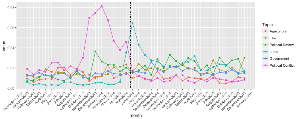
Figure 3: The dotted vertical line represents the May 2014 coup which removed the Pheu Thai government and installed a military government under the authority of the National Council for Peace and Order (NCPO)

Overall, the Political Conflict topic undergoes the most dramatic shift, peaking in the months leading up to the the coup in May 2014. This represents the height of the conflict during the anti-government and anti-election protest by the People’s Democratic Reform Committee (PDRC) which effectively shut down Bangkok in an attempt to oust the Yingluck government and to boycott the election in February. The salience of this topic declines substantially after the military intervened and established a junta government. In contrast, the Junta topic surges after the coup, signaling the media’s attention to the NCPO and the military’s involvement in politics.

Other notable shifts during this transition of power include: (1) a gradual increase in Political Reform which reflects reform-related activities associated with the National Reform Council, National Legislative Assembly and Constitution Drafting Committee, all of which were appointed by the NCPO after the coup; (2) an overall decrease in the topic of Agriculture, reflecting reduced coverage on the rice-pledging scheme of the Yingluck government; (3) a rise in the topic of Law, denoting heightened coverage of anti-corruption and corruption related activities; (4) an increase in Government which denotes greater coverage of government-related activities.

It is plausible that some of these shifts may be attributable to the regime transition. However, without a reliable control group for comparison, it is difficult to make a causal statement regarding the relationship between the regime change and the topic variation observed. Nevertheless, it is possible to conduct a more fine-grained analysis into each topic in order to obtain potentially meaningful descriptive inferences of how topic prevalence and content vary amidst a regime change. See below for a closer look at the frequencies of words over time in documents classified by the model as being highly associated with Political Conflict (Figure 4) and Junta (Figure 5).

### Attach most associated topic to each document
nation.topics.df <- as.data.frame(nation.topics)
nation.topics.df <- transmute(nation.topics.df, doc_id = rownames(nation.topics.df), topic = nation.topics)
nation.topics.df$doc_id <- as.integer(nation.topics.df$doc_id)
df.out <- inner_join(df.2013, nation.topics.df, by = "doc_id")

### Tidy
tidy_df <- df.out %>%
  group_by(topic) %>%
  ungroup() %>%
  unnest_tokens(word, text)

### Word frequencies for selected topics
tidy_df %>% filter(topic == "51") %>% 
  group_by(date) %>%
  summarize(value=n()) %>%
  ggplot(aes(x=date,y=value)) + 
  geom_bar(stat = "identity", fill="skyblue") +
  scale_x_date(date_breaks= "3 month", date_labels = "%B %d, %Y") +
  theme(axis.text.x=element_text(angle=45, hjust=1)) + 
  geom_vline(xintercept = as.numeric(as.Date("2014-05-22")), linetype=4) +
  ggtitle("The Number of Words Written on the ‘Political Conflict’ Topic Per Day")

tidy_df %>% filter(topic == "38") %>% 
  group_by(date) %>%
  summarize(value=n()) %>%
  ggplot(aes(x=date,y=value)) + 
  geom_bar(stat = "identity", fill="skyblue") +
  scale_x_date(date_breaks= "3 month", date_labels = "%B %d, %Y") +
  theme(axis.text.x=element_text(angle=45, hjust=1)) + 
  geom_vline(xintercept = as.numeric(as.Date("2014-05-22")), linetype=4) +
  ggtitle("The Number of Words Written on the ‘Junta’ Topic Per Day")

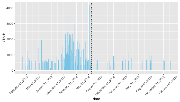
Figure 4: The Number of Words Written on the "Political Conflict" Topic Per Day

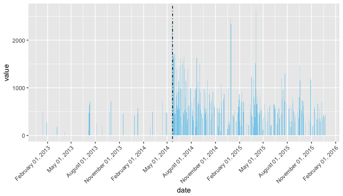
Figure 5: The Number of Words Written on the "Junta" Topic Per Day

Sentiment Analysis

How do sentiments differ prior to and after the coup? Using the bing lexicon which classifies words as positive or negative, I compute unigram sentiment scores for the following topics: Agriculture, Law, Political Reform, Junta, Government and Political Conflict. For corpus-wide sentiments, see Figure (6). In terms of the variation in sentiments over time, the sentiments associated with the six selected topics are on average more positive after the coup than prior to the coup (Figure 7). This is most clearly illustrated in the plot for Agriculture, Political Conflict, Political Reform and Junta. On the other hand, sentiments on Government are more ambiguous, whereas sentiments on Law are consistently negative.

Sentiment analysis for selected topics

topic.sentiment1  <- tidy_df %>% filter(topic == c("2","24", "33", "38", "46", "51")) %>%
  inner_join(get_sentiments("bing")) %>%
  count(topic, sentiment) %>%
  spread(sentiment, n, fill = 0) %>%
  mutate(sentiment = positive - negative)

topic.sentiment1 %>%
  ggplot(aes(factor(topic, labels=c("Agriculture", "Law", "Political Reform", "Junta", "Government", "Political Conflict")), sentiment)) +
  geom_bar(stat="identity", fill="skyblue3") +
  ylim(-700, 700) +
  xlab("Topic") +
  ylab("Sentiments")

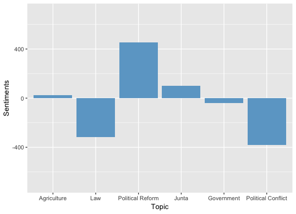
Figure 6: Sentiment Scores for Selected Topics

Sentiment analysis for selected topics over time

topic.sentiment  <- tidy_df %>% filter(topic == c("2","24", "33", "38", "46", "51")) %>%
  inner_join(get_sentiments("bing")) %>%
  count(topic, date, sentiment) %>%
  spread(sentiment, n, fill = 0) %>%
  mutate(sentiment = positive - negative)

ggplot(topic.sentiment, aes(date, sentiment, fill = topic)) +
  geom_col(show.legend = FALSE) + 
  facet_wrap(~factor(topic, labels=c("Agriculture", "Law", "Political Reform", "Junta", "Government", "Political Conflict")), ncol = 2, scales = "free_x") +
  ylab("Sentiments") +
  xlab("Date") +
  ggtitle("Sentiment Analysis")

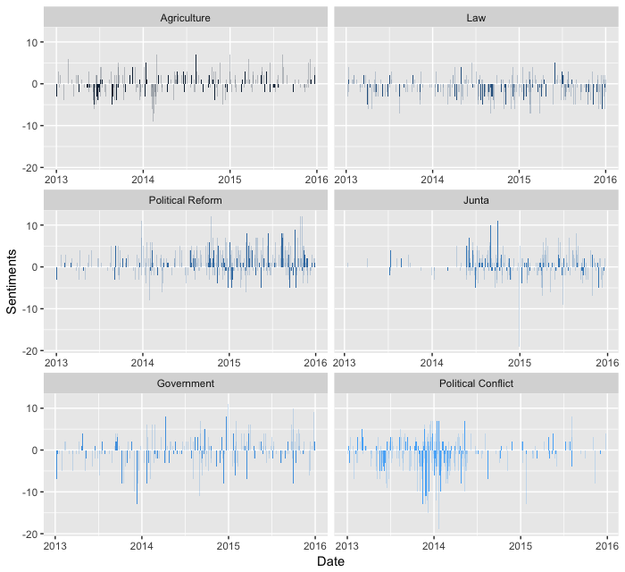
Figure 7: Sentiment Variation Over Time

On average, sentiments for the six selected topics are more positive after the coup than prior to the coup. This is most clearly illustrated in the plot for Agriculture, Political Conflict, Political Reform, and Junta. On the other hand, sentiments on Government are more ambiguous, whereas sentiments on Law are consistently negative.

Prayut vs Yingluck

In this part, I focus on two most prominent political actors, the now-exiled former prime minister Yingluck Shinawatra and the current prime minister and NCPO leader Gen. Prayut Chan-O-Cha. First, I examine the topics that are associated with the names of these two political actors. I find that Yingluck, on the one hand, is associated with Political Conflict, Agriculture, Deep South, Junta and Ministry. Prayut, on the other hand, is associated with Junta, Thailand, Political Reform, Ministry, and Government. Similar to the previous section, I also conduct sentiment analysis on the words that are closely related with the occurrence of the names of Yingluck and Prayut. To do so, I break the newspaper articles into sections of 30 words. Then, I conduct a sentiment analysis on the words within sections that mention Prayut and Yingluck. Overall, sentiments associated with Yingluck became more negative after the coup, whereas the result is more ambiguous for sentiments associated with Prayut.

### Sentiment Analysis
# Break doc into sections
section_words <- tidy_df %>% 
  group_by(doc_id) %>%
  mutate(section = row_number() %/% 30) %>%
  filter(section > 0) %>%
  filter(!word %in% stop_words$word)

# Yingluck
yingluck_sections <- section_words %>%
  group_by(doc_id, section) %>%
  filter(word=="yingluck") %>%
  select(doc_id, section) %>%
  inner_join(section_words)

yingluck.sentiments  <- yingluck_sections %>%
  inner_join(get_sentiments("bing")) %>%
  count(date, sentiment) %>%
  spread(sentiment, n, fill = 0) %>%
  mutate(sentiment = positive - negative) %>%
  group_by(week = floor_date(date, "week")) %>%
  summarize(value=mean(sentiment))

# Prayut
prayut_sections <- section_words %>%
  group_by(doc_id, section) %>%
  filter(word == "prayut"|word == "prayuth") %>%
  select(doc_id, section) %>%
  inner_join(section_words)

prayut.sentiments  <- prayut_sections %>%
  inner_join(get_sentiments("bing")) %>%
  count(date, sentiment) %>%
  spread(sentiment, n, fill = 0) %>%
  mutate(sentiment = positive - negative) %>%
  group_by(week = floor_date(date, "week")) %>%
  summarize(value=mean(sentiment))

# Graph
yingluck.sentiments$label <- "Yingluck"
prayut.sentiments$label <- "Prayut"
yingluck.vs.prayut <- full_join(yingluck.sentiments, prayut.sentiments)

ggplot(yingluck.vs.prayut, aes(week, value, col=label)) +
  geom_line() +
  theme_classic() +
  scale_x_date(date_breaks= "3 month", date_labels = "%b %Y") +
  theme(axis.text.x=element_text(angle=45, hjust=1)) + 
  geom_vline(xintercept = as.numeric(as.Date("2014-05-22")), linetype=4) +
  geom_hline(yintercept = 0, size=0.1) +
  theme(legend.position = "bottom", legend.title=element_blank()) +
  xlab("Date") +
  ylab("Sentiment") +
  scale_color_manual(values=c("#9999CC", "#CC6666"))

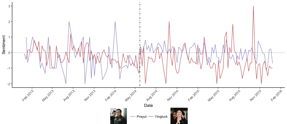
Figure 8: Sentiment Scores for Prayut and Yingluck (Weekly Averages)

### Top Topics associated with Yingluck and Prayut
tidy(mod.out.60) %>%
  filter(term == "yingluck") %>%
  top_n(10, beta) %>%
  arrange(-beta) %>%
  ggplot(aes(x=reorder(topic, -beta), y=beta)) +
  geom_bar(stat="identity", fill="tomato2") +
  coord_flip()

tidy(mod.out.60) %>%
  filter(term == "prayut"|term == "prayuth") %>%
  top_n(20, beta) %>%
  arrange(-beta) %>%
  ggplot(aes(x=reorder(topic, -beta), y=beta)) +
  geom_bar(stat="identity", fill="darkgreen")

### Table
topic_list <- data.frame(t(nation.terms))
topic_list <- within(topic_list, x <- paste(X1, X2, X3, X4, X5, X6, X7, X8, X9, X10, sep=", ")) %>% select(x)
colnames(topic_list) <- NULL
topic_list <- tibble::rownames_to_column(topic_list)
colnames(topic_list) <- c("Topic", "Keys")

yingluck.pattern <- tidy(mod.out.60) %>%
  filter(term == "yingluck") %>%
  top_n(5, beta) %>%
  arrange(-beta) %>%
  select(topic)

prayut.pattern <- tidy(mod.out.60) %>%
  filter(term == "prayut") %>%
  top_n(5, beta) %>%
  arrange(-beta) %>%
  select(topic)

Topic	Keys
Topic 51	protest, polit, yingluck, govern, thaksin, shinawatra, democrat, minist, thai, parti
Topic 2	rice, farmer, price, tonn, govern, scheme, agricultur, million, export, rubber
Topic 18	peac, muslim, group, south, talk, thai, insurg, govern, islam, secur
Topic 38	prayut, minist, militari, prime, general, junta, ncpo, coup, chanocha, order
Topic 20	ministri, said, govern, minist, plan, nation, state, committe, budget, will

Top 5 Topics Associated with Yingluck Shinawatra

Topic	Keys
Topic 38	prayut, minist, militari, prime, general, junta, ncpo, coup, chanocha, order
Topic 50	thailand, one, can, peopl, thai, will, like, letter, mani, just
Topic 33	elect, reform, constitut, polit, vote, parti, charter, member, new, nation
Topic 20	ministri, said, govern, minist, plan, nation, state, committe, budget, will
Topic 46	govern, countri, corrupt, polici, public, need, reform, thailand, nation, system

Top 5 Topics Associated with Prayut Chan-o-cha

Conclusion

To conclude, the study reveals striking differences between newspaper articles that were published prior to and after the military takeover in May 2014 with regards to both topic prevalence and content within the topics identified by the model. However, it must be emphasized that this finding is merely descriptive, not causal. Further work is required in order to falsify or substantiate a causal interpretation of the observed differences which, in theory, could be due to a range of other factors beyond regime transition. Future studies should aim to incorporate a control group that is suitable for comparison and for ruling out potential confounding variables. Furthermore, even when the findings are robust, the difficulty of interpreting the variation in topic prevalence and content remains. Thus, theory development with regards to the relationship between regime transition and the media is necessary to spell out the mechanisms through which changes in political institutions and rules of the game translate into changes in public opinions and sentiments as reflected by the media.

In terms of the methodology, future work should improve upon the current dictionary-based method for document selection in order to reduce the number of false positives and produce a more reliable topic model with greater semantic validity. In addition, the topic model in this study makes modeling assumptions regarding the exchangeability of words and the static nature of topics over time. Implementing a topic model that accounts for the importance of word ordering (Wallach 2006) and the dynamic nature of topics (Blei and Lafferty 2006) would contribute to a more realistic representation of the latent topics and their variation in response to the regime transition. Finally, incorporating other news outlet, in particular those with different political leanings and those that are free from media censorship in Thailand, would offer additional analytical leverage both for inferring whether variation in topics and contents can be attributed to regime transition and for generating externally valid claims regarding the media and regime change.

Bibliography

Arun, Rajkumar, Venkatasubramaniyan Suresh, CE Veni Madhavan, and MN Narasimha Murthy. “On Finding the Natural Number of Topics with Latent Dirichlet Allocation: Some Observations.” In Pacific-Asia Conference on Knowledge Discovery and Data Mining, 391–402. Springer, 2010.

Blei, David M., and John D. Lafferty. “Dynamic Topic Models.” In Proceedings of the 23rd International Conference on Machine Learning, 113–120. ACM, 2006.

Blei, David M., Andrew Y. Ng, and Michael I. Jordan. “Latent Dirichlet Allocation.” J. Mach. Learn. Res. 3 (March 2003): 993–1022.

Cao, Juan, Tian Xia, Jintao Li, Yongdong Zhang, and Sheng Tang. “A Density-Based Method for Adaptive LDA Model Selection.” Neurocomputing 72, no. 7–9 (2009): 1775–1781.

Denny, Matthew J., and Arthur Spirling. “Text Preprocessing for Unsupervised Learning: Why It Matters, When It Misleads, and What to Do about It.” Unpublished Manuscript, Dep. Polit. Sci, Stanford Univ and Inst. Quant. Soc. Sci., Harvard Univ. Https://Ssrn. Com/Abstract 2849145 (2017).

Deveaud, Romain, Eric SanJuan, and Patrice Bellot. “Accurate and Effective Latent Concept Modeling for Ad Hoc Information Retrieval.” Document Numérique 17, no. 1 (2014): 61–84.

Griffiths, Thomas L., and Mark Steyvers. “Finding Scientific Topics.” Proceedings of the National Academy of Sciences 101, no. suppl 1 (2004): 5228–5235.

King, Gary, Patrick Lam, and Margaret Roberts. “Computer-Assisted Keyword and Document Set Discovery from Unstructured Text.” American Journal of Political Science, In Press 2017.

Wallach, Hanna M. “Topic Modeling: Beyond Bag-of-Words.” In Proceedings of the 23rd International Conference on Machine Learning, 977–984. ACM, 2006.